
Part 1 and Part 2 both compared data scientists to data analysts. But I’ve been neglecting the unsung heroes of the data world: data engineers. I’m not too familiar with the life of a data engineer. I imagine there’s some overlap with data scientists (Python, Hadoop, etc), but with a stronger emphasis on data infastructure (Spark, AWS, etc.). Coming from a position of complete ignorance, let’s see if we can use NLP to identify the skills that are specific to data engineers. As always, the full code can be found on github.
Data Collection
Similar to Part 1, we’ll extract all data engineer, data scientist and data analyst jobs in London from the Indeed API and then filter out all junior/senior positions and plot the advertised salaries for each job type.
## if you haven't already installed jobbR
# devtools::install_github("dashee87/jobbR")

## loading the packages we'll need
require(jobbR) # searching indeed API
require(dplyr) # data frame filtering/manipulation
require(rvest) # web scraping
require(stringr) # counting patterns within job descriptions
require(plotly) # interactive plots
require(ggplot2) # vanilla plots
require(tm) # text mining
##         job_type num_jobs
## 1 Data Scientist      210
## 2   Data Analyst      158
## 3  Data Engineer      103
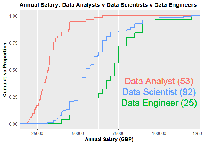
The first thing to note is there are about half as many data engineers posts as there are data scientist posts. Data engineers appear to be paid more than data scientists (though the former is a small sample), with the lowly data analyst bringing up the rear. We’ll now turn our focus to the job description. Repeating the work in Part 2, we’ll plot the proportion of job descriptions that contain specific predefined skills.
Apologies for small text on the x-axis, click here for a better version.
tf-idf
In this post, we’ll attempt to isolate the skills that are more strongly associated with data engineers than data scientists/analysts. We want words that feature frequently in data engineer job descriptions, but rarely with other job types (called term frequency-inverse document frequency, or tf-idf for short).
Firstly, we’ll scrape the job descriptions. I’ve added a few gsub commands to filter out unwanted punctuation features (e.g. bullet points), which may not be detected by the filters within the tm package.
# scrape job description webpages
ds_job_descripts <- unlist(lapply(dataScientists$results.url,
                                  function(x){read_html(x) %>%
                                      html_nodes("#job_summary") %>%
                                      html_text() %>% tolower() %>%
                                      gsub("\n|/"," ",.) %>%
                                      gsub("'|'","",.) %>%
                                      gsub("[^[:alnum:]///' ]", "", .)}))

da_job_descripts <- unlist(lapply(dataAnalysts$results.url,
                                  function(x){read_html(x) %>%
                                      html_nodes("#job_summary") %>%
                                      html_text() %>% tolower()%>%
                                      gsub("\n|/"," ",.) %>%
                                      gsub("'|'","",.) %>%
                                      gsub("[^[:alnum:]///' ]", "", .)}))

de_job_descripts <- unlist(lapply(dataEngineers$results.url,
                                  function(x){read_html(x) %>%
                                      html_nodes("#job_summary") %>%
                                      html_text() %>% tolower() %>%
                                      gsub("\n|/"," ",.) %>%
                                      gsub("'|'","",.) %>%
                                      gsub("[^[:alnum:]///' ]", "", .)}))
Our task consists of two parts:
- Idenitfy words that commonly occur in data engineer job descriptions
- Identify words that commonly occur in data engineer/scientist/analyst job descriptions.
Words that appear highly in the first group but lowly within the second represent skills and themes specific to data engineers. To quantify word frequency, we must convert the job description vectors into a text corpus (large structured set of texts). We remove common words (called stop words) that provide little informative power (e.g. ‘and’, ‘the’, ‘are’). We’ll actually build two seperate corpuses: one for the data engineer jobs descriptions alone (to calculate tf) and another for all of the job descriptions (to calculate idf)).
  de_corpus <- Corpus(VectorSource(de_job_descripts)) %>%
  tm_map(function(x){
    removePunctuation(x, preserve_intra_word_dashes = TRUE)}) %>%
  tm_map(stripWhitespace) %>% tm_map(removeWords,stopwords("english")) %>%
  tm_map(PlainTextDocument)

  all_corpus <- Corpus(VectorSource(c(de_job_descripts,
                                     da_job_descripts,ds_job_descripts))) %>%
  tm_map(function(x){
    removePunctuation(x,preserve_intra_word_dashes = TRUE)}) %>%
  tm_map(stripWhitespace) %>% tm_map(removeWords,stopwords("english")) %>%
  tm_map(PlainTextDocument)
Remember that we’re interested in the frequency of each term within the corpuses. We can easily convert the corpuses to term document matrices, where each row corresponds to an individual term and each column refers to a different job description and the value is simply the number of the times the term appeared in that job description (which is then converted to a binary).
de_tdm <- TermDocumentMatrix(de_corpus)
all_tdm <- TermDocumentMatrix(all_corpus)
de_df <- data.frame(word= row.names(de_tdm),
                 tf = rowSums(ifelse(as.matrix(de_tdm)>0,1,0)),
                 row.names = NULL, stringsAsFactors = FALSE)
all_df <- data.frame(word= row.names(all_tdm),
                 tf = rowSums(ifelse(as.matrix(all_tdm)>0,1,0)),
                 row.names = NULL, stringsAsFactors = FALSE)
# data engineer common words
de_df %>% arrange(-tf) %>% head
##         word  tf
## 1       data 103
## 2 experience  90
## 3   engineer  85
## 4       will  83
## 5    working  80
## 6       team  71
# all jobs common words
all_df %>% arrange(-tf) %>% head
##         word  tf
## 1       data 469
## 2 experience 412
## 3       will 386
## 4     skills 346
## 5       team 342
## 6       work 314
Taking the term frequency (tf) alone, unsurprisingly, we see that ‘data’ and ‘engineer’ are two of the three most common words in data engineer job descriptions. The remaining terms are more generic, illustrated by their high ranking among all jobs. This demonstrates the importance of the inverse document frequency (idf) component. It will penalise terms such as ‘skills’, ‘team’ and ‘work’, as they’re not strongly associated with data engineers exclusively. We’ll normalise the tf score (divide by the max) and calculate the idf. The tf_idf is simply the product of the tf and idf.
de_df$tf = de_df$tf/max(de_df$tf)
de_idf <- data.frame(word=row.names(all_tdm),
               idf = log2(length(all_corpus)/rowSums(
                 ifelse(as.matrix(all_tdm)>0,1,0))),
               row.names = NULL, stringsAsFactors = FALSE)
de_df$tf_idf = de_df$tf * de_idf[match(de_df$word,de_idf$word),]$idf
knitr::kable(de_df %>% inner_join(de_idf,by=c("word"="word")) %>%
               arrange(-tf_idf) %>% mutate(rank=row_number()) %>%
               select(rank,word,tf,idf,tf_idf)  %>% head(40), digits=3)
| rank | word | tf | idf | tf_idf |
|---|---|---|---|---|
| 1 | engineer | 0.825 | 2.372 | 1.957 |
| 2 | etl | 0.330 | 3.388 | 1.118 |
| 3 | engineers | 0.330 | 3.236 | 1.068 |
| 4 | spark | 0.544 | 1.949 | 1.060 |
| 5 | java | 0.379 | 2.690 | 1.018 |
| 6 | aws | 0.311 | 3.265 | 1.014 |
| 7 | pipelines | 0.262 | 3.750 | 0.983 |
| 8 | engineering | 0.485 | 1.997 | 0.969 |
| 9 | hadoop | 0.495 | 1.925 | 0.953 |
| 10 | scala | 0.330 | 2.835 | 0.936 |
| 11 | platform | 0.359 | 2.576 | 0.925 |
| 12 | design | 0.515 | 1.782 | 0.917 |
| 13 | architecture | 0.252 | 3.558 | 0.898 |
| 14 | technologies | 0.427 | 2.034 | 0.869 |
| 15 | big | 0.534 | 1.603 | 0.856 |
| 16 | software | 0.369 | 2.295 | 0.847 |
| 17 | linux | 0.204 | 4.022 | 0.820 |
| 18 | infrastructure | 0.223 | 3.632 | 0.811 |
| 19 | redshift | 0.194 | 4.125 | 0.801 |
| 20 | systems | 0.437 | 1.824 | 0.797 |
| 21 | technical | 0.437 | 1.792 | 0.783 |
| 22 | nosql | 0.243 | 3.125 | 0.758 |
| 23 | hands | 0.204 | 3.710 | 0.756 |
| 24 | years | 0.388 | 1.937 | 0.752 |
| 25 | web | 0.262 | 2.835 | 0.743 |
| 26 | kafka | 0.165 | 4.487 | 0.741 |
| 27 | cloud | 0.204 | 3.632 | 0.740 |
| 28 | applications | 0.291 | 2.487 | 0.724 |
| 29 | building | 0.340 | 2.111 | 0.717 |
| 30 | environments | 0.194 | 3.632 | 0.705 |
| 31 | databases | 0.262 | 2.690 | 0.705 |
| 32 | date | 0.233 | 2.973 | 0.693 |
| 33 | languages | 0.262 | 2.632 | 0.690 |
| 34 | mapreduce | 0.165 | 4.179 | 0.690 |
| 35 | pig | 0.175 | 3.925 | 0.686 |
| 36 | hive | 0.252 | 2.710 | 0.684 |
| 37 | scripting | 0.194 | 3.522 | 0.684 |
| 38 | production | 0.214 | 3.152 | 0.673 |
| 39 | processes | 0.262 | 2.487 | 0.652 |
| 40 | build | 0.408 | 1.576 | 0.643 |
It’s a good sanity check that ‘engineer’ returned the highest tf_idf score, as we’d expect that to be relatively specific to data engineer job descriptions. Also, it’s reassuring that the generic terms that previously scored well (e.g. ‘data’, ‘team’, ‘will’) are not in the table. The table provides some interesting insights. Take the example of ‘spark’: it has a relatively high tf, but is penalised by a low idf (spark is also a key skill among data scientists). ‘etl’, on the other hand, has a considerably lower tf, but outranks spark due to its higher idf (etl is a term more uniquely associated with data engineers).
It’s important to note that there is no strict defintion of either tf or idf. If you wish, you can attach more importance to either by applying a particular variant (a few examples here). I suppose it depends whether you think terms like ‘spark’ (high tf; low idf) should rank more highly than terms like ‘etl’ (low tf; high idf).
Summary
After some exploratory analysis, we used term frequency-inverse document frequency to idenitfy words and skills that are uniquely associated with data engineers. Think of the output as potential conversation starters with your engineer counterparts. “So… how about that etl?”
Leave a Comment