
As my father once told me: ‘If you don’t get the job, at least get a blog post’. This post was motivated by a task I was given for a data scientist job, which involved predicting road accidents in the UK. I won’t focus on the specific task (that would encourage cheating), but instead will explore the rich dataset and use ARIMA to predict the number of road accidents in 2016 (as always, the full code is posted on github).
Getting the Data
If an injury occurs in a road accident that was reported to the police, they produce a detailed report (age/sex of casualties, vehicle/road types, etc). These reports, going back to 2005, are collated and compiled within multiple csvs, which are freely available online (here). They are well formatted: missing data is marked; tidy columns with relatively intuitive names. The csvs are quite big and combined in zip files; you’ll need to download them to your computer and then extract the csvs. Note that the 2015 must be downloaded separately, while the 2005-2014 data is available under the 2014 tab. Okay, so let’s get started.
# loading the packages we'll need
library(dplyr) # data manipulation/filtering
library(ggplot2) # vanilla graphs
library(plotly) # interactive graphs
library(lubridate) # time manipulation functions
library(zoo) # some more time manipulation functions
library(forecast) # time series forecasting
library(RCurl) # import Dow Jones data
library(tseries) # time series statistical analysis

options(stringsAsFactors = FALSE)

# accidents file
tot_accs = rbind(read.csv("/Accidents0514.csv") %>%
                   rename_("Accidents_2015.csv")) %>%
  mutate(Date=as.POSIXct(Date, format="%d/%m/%Y"))

# casualties file
tot_cas= rbind(read.csv("/Casualties0514.csv") %>%
                  rename_("Accident_Index" ="ï..Accident_Index"),
 read.csv("/Casualties_2015.csv") %>%
   select(-Casualty_IMD_Decile))

# vehicles file
tot_veh= rbind(read.csv("/Vehicles0514.csv") %>%
                  rename_("Accident_Index" ="ï..Accident_Index"),
 read.csv("/Vehicles_2015.csv") %>%
   select(-Vehicle_IMD_Decile))
We now have three datasets: Accidents (time and location of accident, road type, weather conditions, etc); Casualties (age, sex, driver/passenger status, severity, etc); Vehicle (type, engine capacity, etc). We’ll start off with some minor exploration of the data.
# looking at the structure of the datasets
 explore_data=as.data.frame(t(sapply(list(tot_accs,tot_cas,tot_veh),function(x){
  c(length(unique(x$Accident_Index)),
    length(x),
    nrow(x))
})))

colnames(explore_data)=c("# Accidents", "# Columns","# Rows")
rownames(explore_data)=c("Accidents File","casualties File","Vehicles File")
explore_data
##                 # Accidents # Columns  # Rows
## Accidents File      1780653        32 1780653
## casualties File     1780653        15 2402909
## Vehicles File       1780653        22 3262270
One reassuring feature is that all files have the same number of accidents, which suggests the datasets could be easily joined on the accident number. The accidents file has the most columns, while the vehicles file has the most rows (one row for each vehicle involved in the accident). Let’s continue the exploratory analysis by addressing the question that has long divided mankind: Are men better drivers than women?
# Drivers in road accidents split by sex
tot_veh %>% group_by(Sex_of_Driver) %>% summarize(num_accs=n()) %>%
  mutate(Sex_of_Driver=c("Data Missing","Male","Female","Unknown")) %>%
  mutate(prop=paste(round(100*num_accs/sum(num_accs),2),"%"))
## # A tibble: 4 × 3
##   Sex_of_Driver num_accs    prop
##           <chr>    <int>   <chr>
## 1  Data Missing       52     0 %
## 2          Male  2147401 65.83 %
## 3        Female   924565 28.34 %
## 4       Unknown   190252  5.83 %
The data suggests that women are less likely to be drivers in a road accident. I suppose there are two possible explanations for this: women are better drivers or there are significantly less female drivers on the road generally speaking. There is some evidence to support the latter theory, but not enough to discount the notion that men are simply worse drivers. Well, worse isn’t really the right word, men tend to take more risks in life and that includes driving.
Having settled one of the most contentious issues around (next up, the Syrian Civil War), let’s look at distribution of road accidents across the week.
# number of road accidents by day of the week
tot_accs %>% group_by(Day_of_Week) %>% summarize(num_accs=n()) %>%
  mutate(Day_of_Week=c("Sunday","Monday","Tuesday","Wednesday",
                       "Thursday","Friday","Saturday")) %>%
  mutate(prop=paste(round(100*num_accs/sum(num_accs),2),"%"))
## # A tibble: 7 × 3
##   Day_of_Week num_accs    prop
##         <chr>    <int>   <chr>
## 1      Sunday   195326 10.97 %
## 2      Monday   253270 14.22 %
## 3     Tuesday   266706 14.98 %
## 4   Wednesday   268390 15.07 %
## 5    Thursday   267494 15.02 %
## 6      Friday   291359 16.36 %
## 7    Saturday   238108 13.37 %
Perhaps unsurprisingly, the quietest day for road accidents is Sunday, while the greatest number of accidents occurs on Friday. Going a level lower, let’s plot the accident time for each day of the week (note: the code for the plots can be found here).
There’s a clear distinction between the weekend and weekdays (though Friday is a sort of hybrid). The weekday rush hour peaks are apparent, while the weekend hits its maximum at around midday, with a noticeable increase in the early morning compared to weekdays. Switching gears, let’s turn our attention to the longer term and plot the number of road accidents per month from 2005-2015.
# just reformatting the days by the yearmonth (e.g. June 2008)
yearlymon_data <- tot_accs %>% group_by(as.yearmon(Date, format="%d/%m/%Y")) %>%
                  summarize(num_accs=n())
colnames(yearlymon_data)[1]="YearMonth"
The good news is that the number of accidents has declined significantly since 2005 (and the UK population increased by nearly 10 % in that time period). You might also detect a seasonal behaviour within the numbers. February typically has the least number of accidents (partly owing to it only have 28/29 days I imagine), while November is the worst month for accidents. So the time series appears to be composed of a trend and cyclical/seasonal component. If we include a noise term to account for random monthly variations, then we should be able to decompose this time series. We’ll opt for a multiplicative model (number accidents is the product of its seasonal/trend/noise components) and use Seasonal and Trend decomposition using Loess (STL) The theory behind time series decomposition is well described here.
# the stl function only takes additive model
# since we want a multiplicative model, we need to first take the log
decomp_accs_ts <- stl(ts(log(yearlymon_data$num_accs),frequency = 12,start=2005),
                      s.window = "periodic")
decomp_accs_ts$time.series <- exp(decomp_accs_ts$time.series)
While the plot illustrates the seasonal behaviour and trend within the data, if we want to forecast the number of accidents in 2016, we’ll employ another form of time series decomposition called Autoregressive Integrated Moving Average (ARIMA). Before we apply ARIMA to our data, we’ll make a little detour and first introduce some of key concepts behind ARIMA.
Stationary Processes And Friends
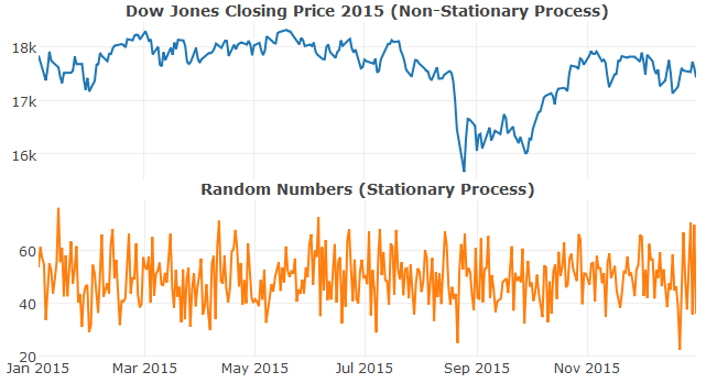
A time series is considered stationary if its statistical properties (mean, variance, etc) are invariant with time. In simple terms, the mean/variance/etc of all subsamples should be approximately identical. A stationary process is quite useful for forecasting: as it contains no trends or longer term changes, knowing its value today is sufficient to predict its future values. This is the principal that underpins ARIMA models.
# importing Dow Jones data for 2015 from yahoo finance
dow_jones <- read.csv(text=getURL(
  "http://chart.finance.yahoo.com/table.csv?s=^DJI&a=0&b=1&c=2015&d=11&e=31&f=2015&g=d&ignore=.csv"),
                      stringsAsFactors = FALSE) %>%
  mutate(Date=as.Date(Date)) %>% arrange(Date)
ARIMA models actually consist of three seperate models, which we’ll now treat in turn, starting with autoregressive models.
Autoregressive Models
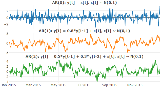
An autoregressive model describes a model where the output is a linear combination of its p previous (or lagged) values, together with a stochastic term (e.g. white noise).
In mathematical terms, an autoregressive model of order p (AR(p)) is written
where denotes the stochastic component in the series. AR(0) is simply uncorrelated noise, while AR(1) represents a Markov process (plotted below).
### Autoregressive Models
set.seed(100)
#AR(0)
ar0 = 0
for(i in 2:365){
  ar0[i] = rnorm(1)}

#AR(1)
ar1 = 0
for(i in 2:365){
  ar1[i] = ar1[i-1]*0.8 + rnorm(1)}

#AR(2)
ar2 = 0
ar2[2] = 0
for(i in 3:365){
  ar2[i] = ar2[i-1]*0.5 + ar2[i-2]*0.3 + rnorm(1)}
Moving Average Models
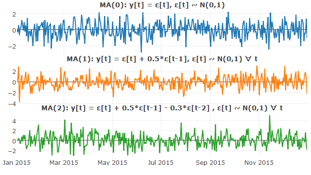
Where autoregressive (AR) models treat output variables as linear combinations of previous values, moving average (MA) models use past forecast errors in a regression-like model.
In mathematical terms, a moving average model of order q (MA(q)) is written
where represents the mean of the series (generally set to 0) and denotes mutually independent stochastic terms.
##### Moving Average Model ######
set.seed(101)
#MA(0)
ma0 = 0
for(i in 2:365){
  ma0[i] = rnorm(1)}

#MA(1)
ma1 = 0
for(i in 2:365){
  ma1[i] = rnorm(1)*0.5 + rnorm(1)}

#MA(2)
ma2 = 0
ma2[2] = 0
for(i in 3:365){
  ma2[i] = rnorm(1)*0.5 - rnorm(1)*0.3 + rnorm(1)}
Okay, so we’ve covered Autoregressive and Moving Average models, the constituents of an ARMA model. But since there’s no I in ARMA, we’re left wondering the significance of that I.
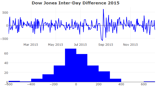
Differencing
The I in ARIMA stands for Integrated and refers to the process of differencing. Non-stationary time series can often be stationarised by taking the difference between successive values. The degree (typically denoted as d) of differencing is simply the number of times the data have had past values subtracted (in practise, at most 2 rounds of differencing is generally required). Going back to the Dow Jones closing price time series, we can tell by eye (and using the augmented dickey-fuller test) that it’s not stationary. However, taking the first difference, the time series has been become stationary (values follow a normal distribution centred near zero).
# augmented Dickey Fuller Test
# not stationary
adf.test(dow_jones$Close)
##
##  Augmented Dickey-Fuller Test
##
## data:  dow_jones$Close
## Dickey-Fuller = -1.9832, Lag order = 6, p-value = 0.5829
## alternative hypothesis: stationary
# stationary
adf.test(diff(dow_jones$Close))
##
##  Augmented Dickey-Fuller Test
##
## data:  diff(dow_jones$Close)
## Dickey-Fuller = -6.9543, Lag order = 6, p-value = 0.01
## alternative hypothesis: stationary
Bringing it all together, non-seasonal ARIMA models are generally denoted ARIMA(p,d,q), where p is the order (number of time lags) of the autoregressive model, d is the degree of differencing and q is the order of the moving-average model. Seasonal models are generally written in form of ARIMA(p,d,q)(P,D,Q)m, where the upper case letters correspond to the seasonal component and m refers to the number of periods per season (12 in our case).
Predicting Number of Road Accidents
Like some people in our dataset, I’ve become a little distracted. Let’s return to our attempt to forecast the number of monthly road accidents in 2016. I’ve spent some time on the theory, but ultimately you just want to know which function to use from which package. Though you can construct an ARIMA model manually (see here for a tutorial), the forecast package includes an auto.arima function, which does all of the hard work for you (determines the appropriate values of p, d and q- though be sure to validate the output, as automated approaches can sometimes throw up strange results).
# fitting ARIMA model to road accident data
acc_arima.fit <- auto.arima(ts(yearlymon_data$num_accs,frequency = 12,start=2005),
                     allowdrift = TRUE, approximation=FALSE)
acc_arima.fit
## Series: ts(yearlymon_data$num_accs, frequency = 12, start = 2005)
## ARIMA(1,1,1)(2,0,0)[12]
##
## Coefficients:
##          ar1      ma1    sar1    sar2
##       0.1492  -0.8702  0.3417  0.4781
## s.e.  0.1054   0.0520  0.0683  0.0748
##
## sigma^2 estimated as 495203:  log likelihood=-1049.7
## AIC=2109.4   AICc=2109.88   BIC=2123.78
The auto.arima function settled on an ARIMA(1,1,1)(2,0,0)12 model for our dataset. We can now quite easily (and hopefully accurately) forecast the number of number of road accidents for the next 12 months.
# forecast road accidents for next 12 months
acc_forecast <- forecast(acc_arima.fit, h=12)
The grey line shows how the ARIMA model compares to the observed 2005-2015 data, while the coloured regions represent the predicted number of accidents in 2016 to varying degrees of certainty. For example, monthly road accidents in 2016 are 80 % and 95 % likely to fall within the green and orange lines, respectively. A monthly value outside of the orange lines would signify an unusually high/low month for road accidents and suggest further investigation for the underlying cause.
Summary
We’ve imported several datasets containing information about road accidents in the UK between 2005 and 2015. After some exploratory analysis and time series theory, we (well, auto.arima) built an ARIMA model to forecast the number of road accidents in 2016. The most interesting part of any predictive model (and any related blog post) is determining how well it performed against the actual data. Unfortunately, this can’t be done until the 2016 data becomes available (probably sometime in early 2017). But the good news for me is that I get another blog post by just overlaying the 2016 lines onto the ARIMA graph. This blog stuff pretty much writes itself.
Leave a Comment