
In an earlier post, I showed how to build a simple Poisson model to crudely predict the outcome of football (soccer) matches. In the same way teams herald slight changes to their traditional plain coloured jerseys as ground breaking (And this racing stripe here I feel is pretty sharp), I thought I’d show how that basic model could be tweaked and improved in order to achieve revolutionary status.
The changes are motivated by a combination of intuition and statistics. The Dixon-Coles model (named after the paper’s authors) corrects for the basic model’s underestimation of draws and it also incorporates a time component so that recent matches are considered more important in calculating average goals rate. This isn’t a particularly novel idea for a blog post. There are numerous implementation of the Dixon-Coles model out there. Like any somewhat niche statistical modelling exercise, however, they are mostly available in R. I strongly recommend the excellent opisthokonta blog, especially if you’re interested in more advanced models. If you’re not interested in the theory and just want to start making predictions with R, then check out the regista package on GitHub.
As always, the corresponding Jupyter notebook can be downloaded from my GitHub. I’ve also uploaded some Python files, if you’d prefer to skip the highly engaging commentary.
Data
We’ll initially pull the match results for the EPL 2017/18 season from football-data.co.uk. This code is pretty much the same as last time.
import pandas as pd
import matplotlib.pyplot as plt
import numpy as np
import seaborn as sns
from scipy.stats import poisson,skellam
from scipy.optimize import minimize

epl_1718 = pd.read_csv("http://www.football-data.co.uk/mmz4281/1718/E0.csv")
epl_1718 = epl_1718[['HomeTeam','AwayTeam','FTHG','FTAG']]
epl_1718 = epl_1718.rename(columns={'FTHG': 'HomeGoals', 'FTAG': 'AwayGoals'})
epl_1718.head()
| HomeTeam | AwayTeam | HomeGoals | AwayGoals | |
|---|---|---|---|---|
| 0 | Arsenal | Leicester | 4 | 3 |
| 1 | Brighton | Man City | 0 | 2 |
| 2 | Chelsea | Burnley | 2 | 3 |
| 3 | Crystal Palace | Huddersfield | 0 | 3 |
| 4 | Everton | Stoke | 1 | 0 |
Basic Poisson Model
I won’t spend too long on this model, as it was the subject of the previous post. Essentially, you treat the number of goals scored by each team as two independent Poisson distributions (henceforth called the Basic Poisson (BP) model). The shape of each distribution is determined by the average number of goals scored by that team. A little reminder on the mathematical definition of the Poisson distribution:
In our case, represents the team’s average or expected goal scoring rate. The Poisson distribution is a decent approximation of a team’s scoring frequency. All of the model’s discussed here agree on this point; the disagreement centres on how to calculate and .
We can formulate the model in mathematical terms:
In this equation, and refer to the home and away teams, respectively; and denote each team’s attack and defensive strength, respectively, while represents the home advantage factor. So, we need to calculate and for each team, as well as (the home field advantage term- it’s the same value for every team). As this was explained in the previous post, I’ll just show the model output.
                 Generalized Linear Model Regression Results
==============================================================================
Dep. Variable:                  goals   No. Observations:                  760
Model:                            GLM   Df Residuals:                      720
Model Family:                 Poisson   Df Model:                           39
Link Function:                    log   Scale:                             1.0
Method:                          IRLS   Log-Likelihood:                -1052.3
Date:                Thu, 13 Sep 2018   Deviance:                       796.97
Time:                        09:24:25   Pearson chi2:                     683.
No. Iterations:                     5
==============================================================================================
                                 coef    std err          z      P>|z|      [0.025      0.975]
----------------------------------------------------------------------------------------------
Intercept                      0.5427      0.189      2.878      0.004       0.173       0.912
team[T.Bournemouth]           -0.4886      0.189     -2.580      0.010      -0.860      -0.117
team[T.Brighton]              -0.7769      0.207     -3.745      0.000      -1.183      -0.370
team[T.Burnley]               -0.7349      0.203     -3.612      0.000      -1.134      -0.336
team[T.Chelsea]               -0.1912      0.172     -1.109      0.268      -0.529       0.147
team[T.Crystal Palace]        -0.4949      0.189     -2.614      0.009      -0.866      -0.124
team[T.Everton]               -0.5143      0.191     -2.697      0.007      -0.888      -0.141
team[T.Huddersfield]          -0.9673      0.222     -4.354      0.000      -1.403      -0.532
team[T.Leicester]             -0.2703      0.177     -1.523      0.128      -0.618       0.078
team[T.Liverpool]              0.1134      0.160      0.710      0.478      -0.200       0.426
team[T.Man City]               0.3351      0.152      2.208      0.027       0.038       0.633
team[T.Man United]            -0.1090      0.168     -0.648      0.517      -0.439       0.221
team[T.Newcastle]             -0.6466      0.198     -3.263      0.001      -1.035      -0.258
team[T.Southampton]           -0.6901      0.202     -3.422      0.001      -1.085      -0.295
team[T.Stoke]                 -0.7334      0.205     -3.569      0.000      -1.136      -0.331
team[T.Swansea]               -0.9693      0.222     -4.364      0.000      -1.405      -0.534
team[T.Tottenham]             -0.0159      0.165     -0.096      0.923      -0.339       0.307
team[T.Watford]               -0.5080      0.191     -2.664      0.008      -0.882      -0.134
team[T.West Brom]             -0.8674      0.214     -4.049      0.000      -1.287      -0.448
team[T.West Ham]              -0.4165      0.186     -2.243      0.025      -0.780      -0.053
opponent[T.Bournemouth]        0.1491      0.190      0.784      0.433      -0.224       0.522
opponent[T.Brighton]           0.0155      0.196      0.079      0.937      -0.368       0.399
opponent[T.Burnley]           -0.3084      0.213     -1.448      0.148      -0.726       0.109
opponent[T.Chelsea]           -0.3079      0.215     -1.434      0.152      -0.729       0.113
opponent[T.Crystal Palace]     0.0452      0.195      0.232      0.816      -0.336       0.427
opponent[T.Everton]            0.0974      0.192      0.507      0.612      -0.279       0.474
opponent[T.Huddersfield]       0.0809      0.192      0.421      0.674      -0.296       0.458
opponent[T.Leicester]          0.1440      0.191      0.755      0.450      -0.230       0.518
opponent[T.Liverpool]         -0.2847      0.215     -1.326      0.185      -0.706       0.136
opponent[T.Man City]          -0.6041      0.238     -2.534      0.011      -1.071      -0.137
opponent[T.Man United]        -0.6077      0.236     -2.580      0.010      -1.069      -0.146
opponent[T.Newcastle]         -0.1185      0.203     -0.585      0.558      -0.515       0.278
opponent[T.Southampton]        0.0550      0.194      0.284      0.777      -0.325       0.435
opponent[T.Stoke]              0.2476      0.186      1.334      0.182      -0.116       0.611
opponent[T.Swansea]            0.0458      0.194      0.236      0.813      -0.334       0.426
opponent[T.Tottenham]         -0.3495      0.218     -1.603      0.109      -0.777       0.078
opponent[T.Watford]            0.1962      0.188      1.043      0.297      -0.172       0.565
opponent[T.West Brom]          0.0489      0.194      0.252      0.801      -0.331       0.429
opponent[T.West Ham]           0.2612      0.186      1.407      0.159      -0.103       0.625
home                           0.2888      0.063      4.560      0.000       0.165       0.413
==============================================================================================
poisson_model.predict(pd.DataFrame(data={'team': 'Arsenal', 'opponent': 'Southampton',
                                       'home':1},index=[1]))
1    2.426661
dtype: float64
poisson_model.predict(pd.DataFrame(data={'team': 'Southampton', 'opponent': 'Arsenal',
                                       'home':0},index=[1]))
1    0.862952
dtype: float64
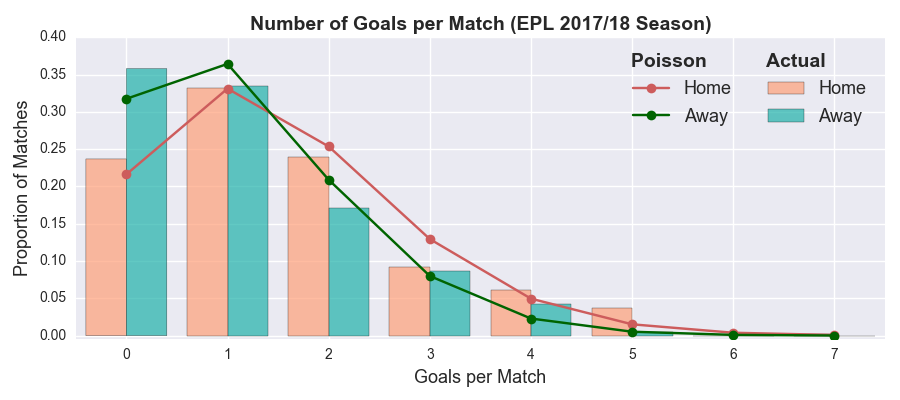
As an example, Arsenal (playing at home) would be expected to score 2.43 goals against Southampton, while their opponents would get about 0.86 goals on average (I’m using the terms average and expected interchangeably). As each team is treated independently, we can construct a match score probability matrix.
First published by Maher in 1982, the BP model still serves a good starting point from which you can add features that more closely reflect the reality. That brings us onto the Dixon-Coles (DC) model.
Dixon-Coles Model
In their 1997 paper, Mark Dixon and Stuart Coles proposed two specific improvements to the BP model:
- Introduce an interaction term to correct underestimated frequency of low scoring matches
- Apply time decay component so that recent matches are weighted more strongly
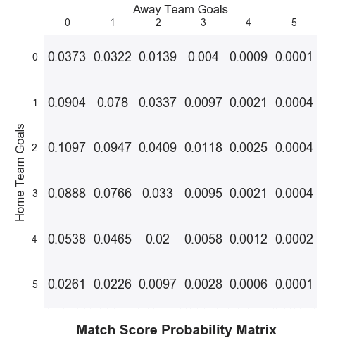
The authors claim that low score results (0-0, 1-0, 0-1 and 1-1) are inherently under-reported by the BP model. In the paper, they provide some analysis that supports their case- though I wouldn’t call their approach particularly rigorous. The matrix below shows the average difference between actual and model predicted scorelines for the 2005/06 season all the way up to the 2017/18 season. Green cells imply the model underestimated those scorelines, while red cells suggest overestimation- the colour strength indicates the level of disagreement.
There does seem to be an issue around low scoring draws, though it is less apparent with 1-0 and 0-1 results. The Dixon-Coles (DC) model applies a correction to the BP model. It can be written in these mathematical terms:
The key difference over the BP model is the addition of the (tau) function. It is highly dependent on the (rho) parameter, which controls the strength of the correction (note: setting =0 equates to the standard BP model). We can easily convert to Python code.
def rho_correction(x, y, lambda_x, mu_y, rho):
    if x==0 and y==0:
        return 1- (lambda_x * mu_y * rho)
    elif x==0 and y==1:
        return 1 + (lambda_x * rho)
    elif x==1 and y==0:
        return 1 + (mu_y * rho)
    elif x==1 and y==1:
        return 1 - rho
    else:
        return 1.0
Unfortunately, you can’t just update your match score matrix with this function; you need to recalculate the various coefficients that go into the model. And unfortunately again, you can’t just implement an off the shelf generalised linear model, as we did before. We have to construct the likelihood function and find the coefficients that maximise it- a technique known as Maximum Likelihood Estimation. With matches indexed and corresponding scores (, ), this is the likelihood function that we seek to maximise:
In this equation, and respectively denote the indices of the home and away teams in match . For a few different reasons (numerical precision, practicality, etc.), we’ll actually maximise the log-likelihood function. As the logarithm is a strictly increasing function (i.e. ), both likelihood functions are maximised at the same point. Also, recall that . We can thus write the log-likelihood function in Python code.
def dc_log_like(x, y, alpha_x, beta_x, alpha_y, beta_y, rho, gamma):
    lambda_x, mu_y = np.exp(alpha_x + beta_y + gamma), np.exp(alpha_y + beta_x)
    return (np.log(rho_correction(x, y, lambda_x, mu_y, rho)) +
            np.log(poisson.pmf(x, lambda_x)) + np.log(poisson.pmf(y, mu_y)))
You may have noticed that dc_log_like included a transformation of and , where and , so that we’re essentially trying to calculate expected log goals. This is equivalent to the log link function in the previous BP glm implementation. It shouldn’t really affect model accuracy, it just means that convergence of the maximisation algorithm should be easier as . Non-positive lambdas are not compatible with a Poisson distribution, so this would return warnings and/or errors during implementation.
We’re now ready to find the parameters that maximise the log likelihood function. Basically, you design a function that takes a set of model parameters as an argument. You set some initial values and potentially include some constraints and select the appropriate optimisation algorithm. I’ve opted for scipy’s minimise function (a possible alternative is fmin- note: the functions seek to minimise the negative log-likelihood). It employs a process analogous to gradient descent, so that the algorithm iteratively converges to the optimal parameter set. The computation can be quite slow as it’s forced to approximate the derivatives. If you’re not as lazy as me, you could potentially speed it up by manually constructing the partial derivatives.
In line with the original Dixon Coles paper and the opisthokonta blog, I’ve added the constraint that (i.e. the average attack strength value is 1). This step isn’t strictly necessary, but it means that it should return a unique solution (otherwise, the model would suffer from overparamterisation and each execution would return different coefficients).
Okay, we’re ready to find the coefficients that maximise the log-likelihood function for the 2017/18 EPL season. The code can be found in the Jupyter notebook. I’ll just display the model parameters.
{'attack_Arsenal': 1.4475654562249061,
 'attack_Bournemouth': 0.95646422693170863,
 'attack_Brighton': 0.68479441389336382,
 'attack_Burnley': 0.69825954509194377,
 'attack_Chelsea': 1.2571663464535701,
 'attack_Crystal Palace': 0.94940962311448773,
 'attack_Everton': 0.93770153726965499,
 'attack_Huddersfield': 0.48932129085135156,
 'attack_Leicester': 1.1898459733738569,
 'attack_Liverpool': 1.5642994035703424,
 'attack_Man City': 1.7860016810986379,
 'attack_Man United': 1.3309554649814161,
 'attack_Newcastle': 0.76698744421411458,
 'attack_Southampton': 0.76528420428466992,
 'attack_Stoke': 0.71957656508258649,
 'attack_Swansea': 0.46646894417565593,
 'attack_Tottenham': 1.4273192933769268,
 'attack_Watford': 0.93387883819783601,
 'attack_West Brom': 0.58374532156356884,
 'attack_West Ham': 1.0449544262494019,
 'defence_Arsenal': -0.90584369881436333,
 'defence_Bournemouth': -0.75848031475781363,
 'defence_Brighton': -0.89464591876906907,
 'defence_Burnley': -1.2267241022008619,
 'defence_Chelsea': -1.2203248942311404,
 'defence_Crystal Palace': -0.85371631529733494,
 'defence_Everton': -0.80976070754509755,
 'defence_Huddersfield': -0.8264653678390087,
 'defence_Leicester': -0.75481859981359867,
 'defence_Liverpool': -1.1755349614996482,
 'defence_Man City': -1.5158390310326799,
 'defence_Man United': -1.5182260478930905,
 'defence_Newcastle': -1.0404285104917514,
 'defence_Southampton': -0.84966692547715239,
 'defence_Stoke': -0.66255356246152519,
 'defence_Swansea': -0.86571839893911184,
 'defence_Tottenham': -1.2719641635656227,
 'defence_Watford': -0.70904298300013313,
 'defence_West Brom': -0.87024534231342454,
 'defence_West Ham': -0.64321365469567715,
 'home_adv': 0.29447553859897918,
 'rho': -0.12851094555265913}
The optimal rho value (-0.1285) returned by the model fits quite nicely with the value (-0.13) given in the equivalent opisthokonta blog post. We can now start making some predictions by constructing match score matrices based on these model parameters. This part is quite similar to BP model, except for the correction applied to the 0-0, 1-0, 0-1 and 1-1 matrix elements.
def dixon_coles_simulate_match(params_dict, homeTeam, awayTeam, max_goals=10):
    team_avgs = [np.exp(params_dict['attack_'+homeTeam] + params_dict['defence_'+awayTeam] + params_dict['home_adv']),
                 np.exp(params_dict['defence_'+homeTeam] + params_dict['attack_'+awayTeam])]
    team_pred = [[poisson.pmf(i, team_avg) for i in range(0, max_goals+1)] for team_avg in team_avgs]
    output_matrix = np.outer(np.array(team_pred[0]), np.array(team_pred[1]))
    correction_matrix = np.array([[rho_correction(home_goals, away_goals, team_avgs[0],
                                                   team_avgs[1], params['rho']) for away_goals in range(2)]
                                   for home_goals in range(2)])
    output_matrix[:2,:2] = output_matrix[:2,:2] * correction_matrix
    return output_matrix
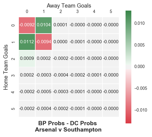
Arsenal Win
Simple Poisson: 0.71846; Dixon-Coles: 0.70951
Southampton Win
Simple Poisson: 0.11446; Dixon-Coles: 0.10437
Draw
Simple Poisson: 0.16703; Dixon-Coles: 0.18608
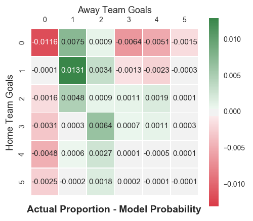
As you can see, the DC model reports a higher probability of a draw compared to the BP model. In fact, you can plot the difference in the match score probability matrices between the two models.
In one way, this is a good plot. The correction was only intended to have an effect on 4 specific match results (0-0, 1-0, 0-1 and 1-1) and that’s what has happened. On the other hand, that was alot of hard work to essentially tweak the existing model. And that’s without even considering whether it was a beneficial adjustment. Without exploring that point any further, I’m going to discuss the second advancement introduced by the DC model.
Dixon-Coles Time Decay Model
Crystal Palace famously (!) lost their opening seven fixtures of the 2017/18 EPL season, conceding 17 times and scoring zero goals. During his short reign, Ronald De Boer had disastrously tried to transform Palace into a more attractive, possession based side. Under their new manager, Roy Hodgson, they returned to their traditional counter attacking style. They recovered well from their poor start to end the season in a respectable 11th place.
Intuitively, if you were trying to predict a Crystal Palace match in January 2018, you would want the model to somewhat discount those losses in August and September 2017. That’s the rationale behind adding a time component to the adjusted Poisson model outlined above. How exactly to down-weight those earlier games is the tricky part. Two weighting options offered in the Dixon-Coles paper are illustrated below.
The first option forces the model to only consider matches within some predefined period (e.g. since the start of the season), while the negative exponential downweights match results more strongly going further into the past. The refined model can be written in these mathematical terms:
where represents the time that match was played, (i.e. set of matches played before time ), , , and are defined as before. represents the non-increasing weighting function. Copying the original Dixon Coles paper, we’ll set to be a negative exponential with rate (called xi). As before, we need to determine the parameters that maximise this likelihood function. We can’t just feed this equation into a minimisation algorithm for various reasons (e.g. we can trivially maximise this function by increasing ). Instead, we’ll fix and determine the remaining parameters the same way as before. We can thus write the corresponding log-likelihood function in the following Python code (recall ). Note how =0 equates to the standard non-time weighted log-likelihood function.
def dc_log_like_decay(x, y, alpha_x, beta_x, alpha_y, beta_y, rho, gamma, t, xi=0):
    lambda_x, mu_y = np.exp(alpha_x + beta_y + gamma), np.exp(alpha_y + beta_x)
    return  np.exp(-xi*t) * (np.log(rho_correction(x, y, lambda_x, mu_y, rho)) +
                              np.log(poisson.pmf(x, lambda_x)) + np.log(poisson.pmf(y, mu_y)))
To determine the optimal value of , we’ll select the model that makes the best predictions. Repeating the process in the Dixon-Coles paper, rather working on match score predictions, the models will be assessed on match result predictions. Essentially, the model that predicted the actual match results with the highest probability will be deemed the winner. An obvious flaw here is that only one match result is considered. For example, if the result was a home win, then the draw and away win probabilities are ignored. Alternative approaches could utilise Ranked Probability Scores or betting probabilities. But we’ll keep things simple and replicate the Dixon Coles paper. We can redefine the objective in mathematical terms; we wish to find that maximises :
This looks more complicated than it really is. The terms just captures the match result e.g. = 1 if match ended in a home win, while the terms are simply the match result probabilities. For example, we can rewrite (probability of home win):
Each of these terms translates to the matrix operations outlined previously. To assess the predictive accuracy of the model, we’ll utilise an approach analogous to the validation set in machine learning. Let’s say we’re trying to predict the fixtures occurring on the 13th January 2018. With fixed to a specific value, we use all of the previous results in that season to build a model. We determine how that model predicted the actual results of those matches with the above equations. We move onto the next set of fixtures (say 20th January) and build the model again- this time including the 13th January games- and assess how well it predicted the results of those matches. We repeat this process for the rest of the 2017/18 season. When we sum up all of these predictions, you have calculated what is called the predicted profile log-likelihood for that value of .
However, a new model must be built for each set of fixtures, so this can be quite slow. I have taken a few steps to speed up the computations:
- Predicting the fixtures for the last 100 days of the 2017/18 EPL season. This is probably preferable anyway, as early season predictions would be quite unreliable.
- Forming match days consisting of three consecutive days (i.e. on Saturday we’ll try to predict matches taking place on Saturday, Sunday and Monday). This should be okay, as teams tend not to play more than once in three days (except at Christmas, which isn’t included in the validation period).
We need to make some slight adjustments to the epl_1718 dataframe to include columns that represent the number of days since the completion of that fixture as well as the match result (home, away or draw).
epl_1718 = pd.read_csv("http://www.football-data.co.uk/mmz4281/1718/E0.csv")
epl_1718['Date'] = pd.to_datetime(epl_1718['Date'],  format='%d/%m/%y')
epl_1718['time_diff'] = (max(epl_1718['Date']) - epl_1718['Date']).dt.days
epl_1718 = epl_1718[['HomeTeam','AwayTeam','FTHG','FTAG', 'FTR', 'time_diff']]
epl_1718 = epl_1718.rename(columns={'FTHG': 'HomeGoals', 'FTAG': 'AwayGoals'})
epl_1718.head()
| HomeTeam | AwayTeam | HomeGoals | AwayGoals | FTR | time_diff | |
|---|---|---|---|---|---|---|
| 0 | Arsenal | Leicester | 4 | 3 | H | 275 |
| 1 | Brighton | Man City | 0 | 2 | A | 274 |
| 2 | Chelsea | Burnley | 2 | 3 | A | 274 |
| 3 | Crystal Palace | Huddersfield | 0 | 3 | A | 274 |
| 4 | Everton | Stoke | 1 | 0 | H | 274 |
With this dataframe, we’re now ready to compare different values of . To speed up this process even further, I made the code parallelisable and ran it across my computer’s multiple (4) cores (see Python file).
It seems that is minimised at =0 (remember that ), which is simply the standard non-weighted DC model. I suppose this makes sense: If you only have data for the season in question, then you don’t have the luxury of down-weighting older results. In the Dixon-Coles paper, they actually compiled data from 4 consecutive seasons (1992/93 to 95/96). You’d expect time weighting to become more effective as the timeframe of your data expands. In other words, the first game of the same season might well be valuable, but the first game of the season five years ago is presumably less valuable. To investigate this hypothesis, we’ll pull data for the previous 5 completed EPL seasons (i.e. 2013/14 to 17/18).
| HomeTeam | AwayTeam | HomeGoals | AwayGoals | FTR | time_diff | |
|---|---|---|---|---|---|---|
| 0 | Arsenal | Aston Villa | 1.0 | 3.0 | A | 1730.0 |
| 1 | Liverpool | Stoke | 1.0 | 0.0 | H | 1730.0 |
| 2 | Norwich | Everton | 2.0 | 2.0 | D | 1730.0 |
| 3 | Sunderland | Fulham | 0.0 | 1.0 | A | 1730.0 |
| 4 | Swansea | Man United | 1.0 | 4.0 | A | 1730.0 |
Same procedure as before, with varying values of , we’ll quanitfy how well the model predicted the match results of the second half of the 17/18 EPL season. Again, I ran the program across multiple cores (see Python file).
Now we have a curve resembles the same function in the Dixon Coles paper. Initially, the model becomes more accurate as you apply a time decay to the historical results. However, at a certain point ( 0.00325), the weighting becomes too harsh and worsens the performance of the model.
The Dixon Coles paper arrived at an optimal =0.0065. However, as they employed half-weeks as their unit of time, we need to divide this value by 3.5. As such, the optimal value here ( = 0.00325) is somewhat higher (note: the opisthokonta blog returned a value of 0.0018, in agreement with the Dixon Coles paper). In this post, I utilised significantly fewer predictions, so it’s possible that a more comparable approach would return a lower .
Another interesting feature of the 5 season graph is that the maximum value of is -125.15. The maximum value of the 1 season is -125.38 (attained at =0). It’s interesting that a data heavy appropriately time-weighted model returned a slightly better level of accuracy than the non-weighted model only using data from that season. That said, the approach outlined here was highly specific (predictions made on one particular season), so I would need to perform more analysis before I would draw any definitive conclusions from this result. Also, as shown in the first post, making predictions towards the end of the season is notoriously difficult, which could also undermine any generalisation of these findings.
Conclusions
We started out by exploring (once again) the basic Poisson model. We then included a bivariate adjustment term to account for the model’s apparent difficulties with low scoring results. Finally, we extended this adjusted model to incorporate a time-decay component, so that older results are considered progressively less important than recent results.
While I’ve described the different models in some detail, I haven’t yet discussed whether these models will make you any money. They won’t.
You can start building your own models with the Jupyter notebook and Python files available from my GitHub account. Thanks for reading!
Leave a Comment