
Football (or soccer to my American readers) is full of clichés: “It’s a game of two halves”, “taking it one game at a time” and “Liverpool have failed to win the Premier League”. You’re less likely to hear “Treating the number of goals scored by each team as independent Poisson processes, statistical modelling suggests that the home team have a 60% chance of winning today”. But this is actually a bit of cliché too (it has been discussed here, here, here and here). As we’ll discover, a simple Poisson model is, well, overly simplistic. But it’s a good starting point and a nice intuitive way to learn about statistical modelling. So, if you came here looking to make money, I hear this guy makes £5000 per month without leaving the house.
Poisson Distribution
The model is founded on the number of goals scored/conceded by each team. Teams that have been higher scorers in the past have a greater likelihood of scoring goals in the future. We’ll import all match results from the recently finished Premier League (2016/17) season. There’s various sources for this data out there (kaggle, football-data.co.uk, github, API). As I built an R wrapper for that API, for purely egotistical (aside: I intially misspelt this as egostistical, which I misread as egostatistical. Unfortunately, egostatistical.com is taken) reasons, we’ll import the data using the fantastic footballR package.
#devtools::install_github("dashee87/footballR") you may need to install footballR
library(footballR)
library(dplyr)
#you'll have to wait to find out the purpose of this mysterious package
library(skellam)
library(ggplot2)
library(purrr)
library(tidyr)
# abettor is an R wrapper for the Betfair API,
# which we'll use to obtain betting odds
#devtools::install_github("phillc73/abettor")
library(abettor)
library(RCurl)

options(stringsAsFactors = FALSE)

# get id for 2016/17 EPL season
epl_id <-fdo_listComps(season = 2016,response = "minified") %>% filter(league=="PL") %>% .$id
# get all matches in 2016/17 EPL season
epl_data <- fdo_listCompFixtures(id = epl_id, response = "minified")$fixtures %>%
  jsonlite::flatten() %>% filter(status=="FINISHED") %>%
  rename(home=homeTeamName, away=awayTeamName, homeGoals=result.goalsHomeTeam,
         awayGoals=result.goalsAwayTeam) %>%
  select(home,away,homeGoals,awayGoals) %>%
# some formatting of team names so that the names returned by footballR are
# compatible with those returned by the Betfair API
  mutate(home=gsub(" FC| AFC|AFC |wich Albion|rystal| Hotspur","",home)) %>%
  mutate(home=ifelse(home=="Manchester United","Man Utd",
                     ifelse(home=="Manchester City","Man City",
                            gsub(" City| United","",home)))) %>%
  mutate(away=gsub(" FC| AFC|AFC |wich Albion|rystal| Hotspur","",away)) %>%
  mutate(away=ifelse(away=="Manchester United","Man Utd",
                             ifelse(away=="Manchester City","Man City",
                                    gsub(" City| United","",away))))
head(epl_data)
##            home      away homeGoals awayGoals
## 1          Hull Leicester         2         1
## 2       Burnley   Swansea         0         1
## 3      C Palace West Brom         0         1
## 4       Everton Tottenham         1         1
## 5 Middlesbrough     Stoke         1         1
## 6   Southampton   Watford         1         1
I’ll omit most of the code that produces the graphs in this post. Don’t worry, you can find that code on my github page. I just presented it here to give you an idea how I formatted the data (mostly dplyr). While that code may look complicated, it mostly involves changing the team names so that they’re compatible with the Betfair API (more on that later). Our task is to model the final round of fixtures in the season, so we must remove the last 10 rows (each gameweek consists of 10 matches).
# remove gameweek 38 from data frame
epl_data <- head(epl_data,-10)
data.frame(avg_home_goals = mean(epl_data$homeGoals),
           avg_away_goals = mean(epl_data$awayGoals))
##   avg_home_goals avg_away_goals
## 1       1.591892       1.183784
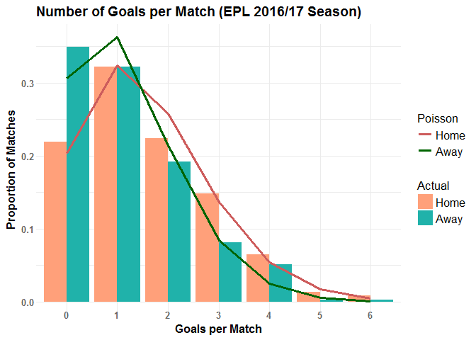
You’ll notice that, on average, the home team scores more goals than the away team. This is the so called ‘home (field) advantage’ (discussed here) and isn’t specific to soccer. This is a convenient time to introduce the Poisson distribution. It’s a discrete probability distribution that describes the probability of the number of events within a specific time period (e.g 90 mins) with a known average rate of occurrence. A key assumption is that the number of events is independent of time. In our context, this means that goals don’t become more/less likely by the number of goals already scored in the match. Instead, the number of goals is expressed purely as function an average rate of goals. If that was unclear, maybe this mathematical formulation will make clearer:
represents the average rate (average number of goals, average number of letters you receive, etc.). So, we can treat the number of goals scored by the home and away team as Poisson distributions. The plot below shows the proportion of goals scored compared to the number of goals estimated by the corresponding Poisson distributions.
We can use this statistical model to estimate the probability of specfic events.
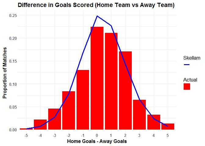
The probability of a draw is simply the sum of the events where the two teams score the same amount of goals.
Note that we consider the number of goals scored by each team to be independent events (i.e. P(A n B) = P(A) P(B)). The difference of two Poisson distribution is actually called a Skellam distribution. So we can calculate the probability of a draw by inputting the mean goal values into this distribution.
# probability of draw between home and away team
skellam::dskellam(0,mean(epl_data$homeGoals),mean(epl_data$awayGoals))
## [1] 0.2480938
# probability of home team winning by one goal
skellam::dskellam(1,mean(epl_data$homeGoals),mean(epl_data$awayGoals))
## [1] 0.2270677
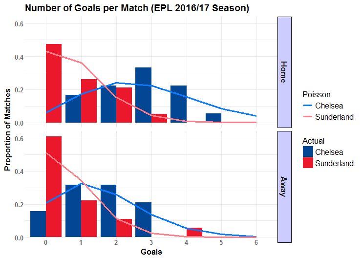
So, hopefully you can see how we can adapt this approach to model specific matches. We just need to know the average number of goals scored by each team and feed this data into a Poisson model. Let’s have a look at the distribution of goals scored by Chelsea and Sunderland (teams who finished 1st and last, respectively).
Building A Model
You should now be convinced that the number of goals scored by each team can be approximated by a Poisson distribution. Due to a relatively sample size (each team plays at most 19 home/away games), the accuracy of this approximation can vary significantly (especially earlier in the season when teams have played fewer games). Similar to before, we could now calculate the probability of various events in this Chelsea Sunderland match. But rather than treat each match separately, we’ll build a more general Poisson regression model (what is that?).
poisson_model <-
rbind(
  data.frame(goals=epl_data$homeGoals,
             team=epl_data$home,
             opponent=epl_data$away,
             home=1),
  data.frame(goals=epl_data$awayGoals,
             team=epl_data$away,
             opponent=epl_data$home,
             home=0)) %>%
glm(goals ~ home + team +opponent, family=poisson(link=log),data=.)
summary(poisson_model)
##
## Call:
## glm(formula = goals ~ home + team + opponent, family = poisson(link = log),
##     data = .)
##
## Deviance Residuals:
##      Min        1Q    Median        3Q       Max
## -2.22652  -1.11951  -0.09455   0.57388   2.59184
##
## Coefficients:
##                       Estimate Std. Error z value Pr(>|z|)
## (Intercept)            0.37246    0.19808   1.880 0.060060 .
## home                   0.29693    0.06315   4.702 2.57e-06 ***
## teamBournemouth       -0.28915    0.17941  -1.612 0.107043
## teamBurnley           -0.64583    0.19994  -3.230 0.001237 **
## teamC Palace          -0.38652    0.18345  -2.107 0.035124 *
## teamChelsea            0.07890    0.16167   0.488 0.625541
## teamEverton           -0.20079    0.17301  -1.161 0.245822
## teamHull              -0.70058    0.20359  -3.441 0.000579 ***
## teamLeicester         -0.42038    0.18696  -2.249 0.024541 *
## teamLiverpool          0.01623    0.16425   0.099 0.921286
## teamMan City           0.01175    0.16423   0.072 0.942976
## teamMan Utd           -0.35724    0.18128  -1.971 0.048767 *
## teamMiddlesbrough     -1.00874    0.22512  -4.481 7.43e-06 ***
## teamSouthampton       -0.58043    0.19504  -2.976 0.002920 **
## teamStoke             -0.60818    0.19660  -3.094 0.001978 **
## teamSunderland        -0.96194    0.22220  -4.329 1.50e-05 ***
## teamSwansea           -0.51364    0.19217  -2.673 0.007522 **
## teamTottenham          0.05319    0.16212   0.328 0.742818
## teamWatford           -0.59688    0.19663  -3.035 0.002401 **
## teamWest Brom         -0.55666    0.19354  -2.876 0.004026 **
## teamWest Ham          -0.48018    0.18943  -2.535 0.011249 *
## opponentBournemouth    0.41095    0.19644   2.092 0.036442 *
## opponentBurnley        0.16565    0.20560   0.806 0.420411
## opponentC Palace       0.32868    0.19956   1.647 0.099554 .
## opponentChelsea       -0.30364    0.23388  -1.298 0.194189
## opponentEverton       -0.04422    0.21838  -0.202 0.839544
## opponentHull           0.49786    0.19263   2.585 0.009751 **
## opponentLeicester      0.33685    0.19887   1.694 0.090289 .
## opponentLiverpool     -0.03744    0.21738  -0.172 0.863250
## opponentMan City      -0.09931    0.22158  -0.448 0.654025
## opponentMan Utd       -0.42197    0.24063  -1.754 0.079494 .
## opponentMiddlesbrough  0.11957    0.20836   0.574 0.566061
## opponentSouthampton    0.04579    0.21138   0.217 0.828496
## opponentStoke          0.22660    0.20315   1.115 0.264667
## opponentSunderland     0.37067    0.19759   1.876 0.060664 .
## opponentSwansea        0.43362    0.19468   2.227 0.025927 *
## opponentTottenham     -0.54307    0.25191  -2.156 0.031099 *
## opponentWatford        0.35330    0.19821   1.782 0.074668 .
## opponentWest Brom      0.09696    0.20935   0.463 0.643248
## opponentWest Ham       0.34851    0.19822   1.758 0.078718 .
## ---
## Signif. codes:  0 '***' 0.001 '**' 0.01 '*' 0.05 '.' 0.1 ' ' 1
##
## (Dispersion parameter for poisson family taken to be 1)
##
##     Null deviance: 973.53  on 739  degrees of freedom
## Residual deviance: 776.11  on 700  degrees of freedom
## AIC: 2164.9
##
## Number of Fisher Scoring iterations: 5
If you’re curious about the glm(...) part, you can find more information here. I’m more interested in the values presented in the Estimate column in the model summary table. This value is similar to the slope in linear regression. Similar to logistic regression, we take the exponent of the parameter values. A positive value implies more goals (), while values closer to zero represent more neutral effects (). First thing you notice is that home has an Estimate of 0.29693. This captures the fact that home teams generally score more goals than the away team (specifically, =1.35 times more likely). But not all teams are created equal. Chelsea has an estimate of 0.07890, while the corresponding value for Sunderland is -0.96194 (sort of saying Chelsea (Sunderland) are better (much worse!) scorers than average). Finally, the opponent* values penalize/reward teams based on the quality of their opposition. This mimics the defensive strength of each team (Chelsea: -0.30364; Sunderland: 0.37067). In other words, you’re less likely to score against Chelsea. Hopefully, that all makes both statistical and intuitive sense.
Let’s start making some predictions for the upcoming match. We simply pass our teams into poisson_model and it’ll return the expected average number of goals for your team (we need to run it twice- we calculate the expected average number of goals for each team separately). So let’s see how many goals we expect Chelsea and Sunderland to score.
predict(poisson_model,
        data.frame(home=1, team="Chelsea",
                   opponent="Sunderland"), type="response")
##        1
## 3.061662
predict(poisson_model,
        data.frame(home=0, team="Sunderland",
                   opponent="Chelsea"), type="response")
##         1
## 0.4093728
Just like before, we have two Poisson distributions. From this, we can calculate the probability of various events. I’ll wrap this in a simulate_match function.
simulate_match <- function(foot_model, homeTeam, awayTeam, max_goals=10){
  home_goals_avg <- predict(foot_model,
                            data.frame(home=1, team=homeTeam,
                                      opponent=awayTeam), type="response")
  away_goals_avg <- predict(foot_model,
                           data.frame(home=0, team=awayTeam,
                                      opponent=homeTeam), type="response")
  dpois(0:max_goals, home_goals_avg) %o% dpois(0:max_goals, away_goals_avg)
}

simulate_match(poisson_model, "Chelsea", "Sunderland", max_goals=4)
##            [,1]       [,2]        [,3]         [,4]         [,5]
## [1,] 0.03108485 0.01272529 0.002604694 0.0003554303 3.637587e-05
## [2,] 0.09517130 0.03896054 0.007974693 0.0010882074 1.113706e-04
## [3,] 0.14569118 0.05964200 0.012207906 0.0016658616 1.704896e-04
## [4,] 0.14868571 0.06086788 0.012458827 0.0017001016 1.739938e-04
## [5,] 0.11380634 0.04658922 0.009536179 0.0013012841 1.331776e-04
This matrix simply shows the probability of Chelsea (rows of the matrix) and Sunderland (matrix columns) scoring a specific number of goals. For example, along the diagonal, both teams score the same the number of goals (e.g. P(0-0)=0.031). So, you can calculate the odds of draw by summing all the diagonal entries. Everything below the diagonal represents a Chelsea victory (e.g P(3-0)=0.149). If you prefer Over/Under markets, you can estimate P(Under 2.5 goals) by summing the entries where the sum of the column number and row number (both starting at zero) is less than 3 (i.e. the 6 values that form the upper left triangle). Luckily, we can use basic matrix manipulation functions to perform these calculations.
chel_sun <- simulate_match(poisson_model, "Chelsea", "Sunderland", max_goals=10)
# chelsea win
sum(chel_sun[lower.tri(chel_sun)])
## [1] 0.8885987
# draw
sum(diag(chel_sun))
## [1] 0.08409349
# sunderland win
sum(chel_sun[upper.tri(chel_sun)])
## [1] 0.02696182
Hmm, our model gives Sunderland a 2.7% chance of winning. But is that right? To assess the accuracy of the predictions, we’ll compare the probabilities returned by our model against the odds offered by the Betfair exchange.
Sports Betting/Trading
Unlike traditional bookmakers, on betting exchanges (and Betfair isn’t the only one- it’s just the biggest), you bet against other people (with Betfair taking a commission on winnings). It acts as a sort of stock market for sports events. And, like a stock market, due to the efficient market hypothesis, the prices available at Betfair reflect the true price/odds of those events happening (in theory anyway). Below, I’ve posted a screenshot of the Betfair exchange on Sunday 21st May (a few hours before those matches started).

The numbers inside the boxes represent the best available prices and the amount available at those prices. The blue boxes signify back bets (i.e. betting that an event will happen- going long using stock market terminology), while the pink boxes represent lay bets (i.e. betting that something won’t happen- i.e. shorting). For example, if we were to bet £100 on Chelsea to win, we would receive the original amount plus 100*1.13= £13 should they win (of course, we would lose our £100 if they didn’t win). Now, how can we compare these prices to the probabilities returned by our model? Well, decimal odds can be converted to the probabilities quite easily: it’s simply the inverse of the decimal odds. For example, the implied probability of Chelsea winning is 1/1.13 (=0.885- our model put the probability at 0.889). I’m focusing on decimal odds, but you might also be familiar with Moneyline (American) Odds (e.g. +200) and fractional odds (e.g. 2/1). The relationship between decimal odds, moneyline and probability is illustrated in the table below. I’ll stick with decimal odds because the alternatives are either unfamiliar to me (Moneyline) or just stupid (fractional odds).
| Match | Home | Draw | Away |
|---|---|---|---|
| Arsenal v Everton | 71.4 % | 17.5 % | 11.6 % |
| Burnley v West Ham | 42 % | 27.8 % | 30.8 % |
| Chelsea v Sunderland | 88.5 % | 8.7 % | 3.4 % |
| Hull v Tottenham | 10.9 % | 17.2 % | 71.9 % |
| Leicester v Bournemouth | 53.5 % | 24.4 % | 23.3 % |
| Liverpool v Middlesbrough | 87.7 % | 9.5 % | 3.6 % |
| Man Utd v C Palace | 41.7 % | 29 % | 29.9 % |
| Southampton v Stoke | 57.1 % | 24.4 % | 19.2 % |
| Swansea v West Brom | 43.1 % | 28.6 % | 29 % |
| Watford v Man City | 5.1 % | 10.2 % | 85.5 % |
So, we have our model probabilities and (if we trust the exchange) we know the true probabilities of each event happening. Ideally, our model would identify situations the market has underestimated the chances of an event occurring (or not occurring in the case of lay bets). For example, in a simple coin toss game, imagine if you were offered $2 for every $1 wagered (plus your stake), if you guessed correctly. The implied probability is 0.333, but any valid model would return a probability of 0.5. The odds returned by our model and the Betfair exchange are compared in the table below.
| Match | Home | Draw | Away | |
|---|---|---|---|---|
| Arsenal v Everton | Betfair | 0.714 | 0.175 | 0.116 |
| Predicted | 0.533 | 0.226 | 0.241 | |
| Difference | 0.181 | -0.051 | -0.125 | |
| Burnley v West Ham | Betfair | 0.42 | 0.278 | 0.308 |
| Predicted | 0.461 | 0.263 | 0.276 | |
| Difference | -0.041 | 0.015 | 0.032 | |
| Chelsea v Sunderland | Betfair | 0.885 | 0.087 | 0.034 |
| Predicted | 0.889 | 0.084 | 0.027 | |
| Difference | -0.004 | 0.003 | 0.007 | |
| Hull v Tottenham | Betfair | 0.109 | 0.172 | 0.719 |
| Predicted | 0.063 | 0.138 | 0.799 | |
| Difference | 0.046 | 0.034 | -0.08 | |
| Leicester v Bournemouth | Betfair | 0.535 | 0.244 | 0.233 |
| Predicted | 0.475 | 0.22 | 0.306 | |
| Difference | 0.06 | 0.024 | -0.073 | |
| Liverpool v Middlesbrough | Betfair | 0.877 | 0.095 | 0.036 |
| Predicted | 0.77 | 0.161 | 0.069 | |
| Difference | 0.107 | -0.066 | -0.033 | |
| Man Utd v C Palace | Betfair | 0.417 | 0.29 | 0.299 |
| Predicted | 0.672 | 0.209 | 0.119 | |
| Difference | -0.255 | 0.081 | 0.18 | |
| Southampton v Stoke | Betfair | 0.571 | 0.244 | 0.192 |
| Predicted | 0.496 | 0.277 | 0.226 | |
| Difference | 0.075 | -0.033 | -0.034 | |
| Swansea v West Brom | Betfair | 0.431 | 0.286 | 0.29 |
| Predicted | 0.368 | 0.266 | 0.366 | |
| Difference | 0.063 | 0.02 | -0.076 | |
| Watford v Man City | Betfair | 0.051 | 0.102 | 0.855 |
| Predicted | 0.167 | 0.203 | 0.631 | |
| Difference | -0.116 | -0.101 | 0.224 | |
Green cells illustrate opportunities to make profitable bets, according to our model (the opacity of the cell is determined by the implied difference). I’ve highlighted the difference between the model and Betfair in absolute terms (the relative difference may be more relevant for any trading strategy). Transparent cells indicate situations where the exchange and our model are in broad agreement. Strong colours imply that either our model is wrong or the exchange is wrong. Given the simplicity of our model, I’d lean towards the latter.
Something’s Poissony
So should we bet the house on Manchester United? Probably not (though they did win!). There’s some non-statistical reasons to resist backing them. Keen football fans would notice that these matches represent the final gameweek of the season. Most teams have very little to play for, meaning that the matches are less predictable (especially when they involve unmotivated ‘bigger’ teams). Compounding that, Man United were set to play Ajax in the Europa Final three days later. Man United manager, Jose Mourinho, had even confirmed that he would rest the first team, saving them for the much more important final. In a similar fashion, injuries/suspensions to key players, managerial sackings would render our model inaccurate. Never underestimate the importance of domain knowledge in statistical modelling/machine learning! We could also think of improvements to the model that would incorporate time when considering previous matches (i.e. more recent matches should be weighted more strongly).
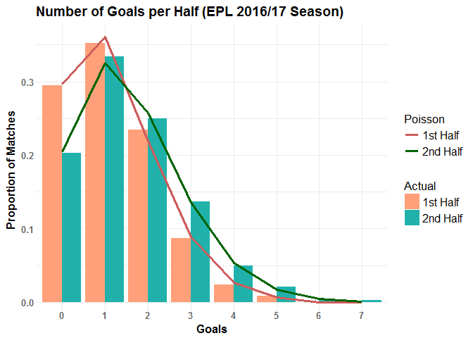
Statistically speaking, is a Poisson distribution even appropriate? Our model was founded on the belief that the number goals can be accurately expressed as a Poisson distribution. If that assumption is misguided, then the model outputs will be unreliable. Given a Poisson distribution with mean , then the number of events in half that time period follows a Poisson distribution with mean /2. In football terms, according to our Poisson model, there should be an equal number of goals in the first and second halves. Unfortunately, that doesn’t appear to hold true.
# the first half goals is missing for a few matches from the API
# so we'll load in a csv instead
epl_1617 <- read.csv(text=getURL("http://www.football-data.co.uk/mmz4281/1617/E0.csv"),
                     stringsAsFactors = FALSE) %>%
  mutate(FHgoals= HTAG+HTHG, SHgoals= FTHG+FTAG-HTAG-HTHG)
We have irrefutable evidence that violates the whole basis of our model, rendering this whole post as pointless as Sunderland!!! Or we can build on our crude first attempt. Rather than a simple univariate Poisson model, we might have more success with a bivariate Poisson distriubtion. The Weibull distribution has also been proposed as a viable alternative. These might be topics for future blog posts.
Summary
We built a simple Poisson model to predict the results of English Premier League matches. Despite its inherent flaws, it recreates several features that would be a necessity for any predictive football model (home advantage, varying offensive strengths and opposition quality). In conclusion, don’t wager the rent money, but it’s a good starting point for more sophisticated realistic models. Thanks for reading!
Leave a Comment