
If you were to pick the three most ridiculous fads of 2017, they would definitely be fidget spinners (are they still cool? Do kids still use that word “cool”?), artificial intelligence and, yes, cryptocurrencies. Joking aside, I’m actually impressed by the underlying concept and I’m quite bullish on the long term prospects of this disruptive technology. But enough about fidget spinners!!! I’m actually not a hodler of any cryptos. So, while I may not have a ticket to the moon, I can at least get on board the hype train by successfully predicting the price of cryptos by harnessing deep learning, machine learning and artificial intelligence (yes, all of them!).
I thought this was a completely unique concept to combine deep learning and cryptos (blog-wise at least), but in researching this post (i.e. looking for code to copy+paste), I came across something quite similar. That post only touched on Bitcoin (the most famous crypto of them all), but I’ll also discuss Ethereum (commonly known as ether, eth or lambo-money). And since Ether is clearly superior to Bitcoin (have you not heard of Metropolis?), this post will definitely be better than that other one.
We’re going to employ a Long Short Term Memory (LSTM) model; it’s a particular type of deep learning model that is well suited to time series data (or any data with temporal/spatial/structural order e.g. movies, sentences, etc.). If you wish to truly understand the underlying theory (what kind of crypto enthusiast are you?), then I’d recommend this blog or this blog or the original (white)paper. As I’m shamelessly trying to appeal to a wider non-machine learning audience, I’ll keep the code to a minimum. There’s a Jupyter (Python) notebook available here, if you want to play around with the data or build your own models. Let’s get started!
Data
Before we build the model, we need to obtain some data for it. There’s a dataset on Kaggle that details minute by minute Bitcoin prices (plus some other factors) for the last few years (featured on that other blog post). Over this timescale, noise could overwhelm the signal, so we’ll opt for daily prices. The issue here is that we may have not sufficient data (we’ll have hundreds of rows rather than thousands or millions). In deep learning, no model can overcome a severe lack of data. I also don’t want to rely on static files, as that’ll complicate the process of updating the model in the future with new data. Instead, we’ll aim to pull data from websites and APIs.
As we’ll be combining multiple cryptos in one model, it’s probably a good idea to pull the data from one source. We’ll use coinmarketcap.com. For now, we’ll only consider Bitcoin and Ether, but it wouldn’t be hard to add the latest overhyped altcoin using this approach. Before we import the data, we must load some python packages that will make our lives so much easier.
import pandas as pd
import time
import seaborn as sns
import matplotlib.pyplot as plt
import datetime
import numpy as np

# get market info for bitcoin from the start of 2016 to the current day
bitcoin_market_info = pd.read_html("https://coinmarketcap.com/currencies/bitcoin/historical-data/?start=20130428&end="+time.strftime("%Y%m%d"))[0]
# convert the date string to the correct date format
bitcoin_market_info = bitcoin_market_info.assign(Date=pd.to_datetime(bitcoin_market_info['Date']))
# when Volume is equal to '-' convert it to 0
bitcoin_market_info.loc[bitcoin_market_info['Volume']=="-",'Volume']=0
# convert to int
bitcoin_market_info['Volume'] = bitcoin_market_info['Volume'].astype('int64')
# look at the first few rows
bitcoin_market_info.head()
| Date | Open | High | Low | Close | Volume | Market Cap | |
|---|---|---|---|---|---|---|---|
| 0 | 2017-11-19 | 7766.03 | 8101.91 | 7694.10 | 8036.49 | 3149320000 | 129595000000 |
| 1 | 2017-11-18 | 7697.21 | 7884.99 | 7463.44 | 7790.15 | 3667190000 | 128425000000 |
| 2 | 2017-11-17 | 7853.57 | 8004.59 | 7561.09 | 7708.99 | 4651670000 | 131026000000 |
| 3 | 2017-11-16 | 7323.24 | 7967.38 | 7176.58 | 7871.69 | 5123810000 | 122164000000 |
| 4 | 2017-11-15 | 6634.76 | 7342.25 | 6634.76 | 7315.54 | 4200880000 | 110667000000 |
To explain what’s just happened, we’ve loaded some python packages and then imported the table that you see on this site. With a little bit of data cleaning, we arrive at the above table. We also do the same thing for ether by simply replacing ‘bitcoin’ with ‘ethereum’ in the url (code omitted).
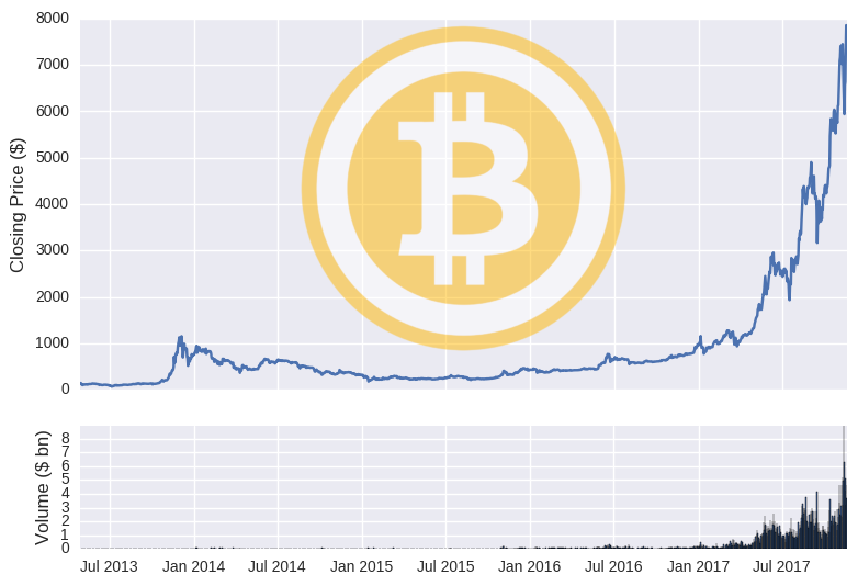
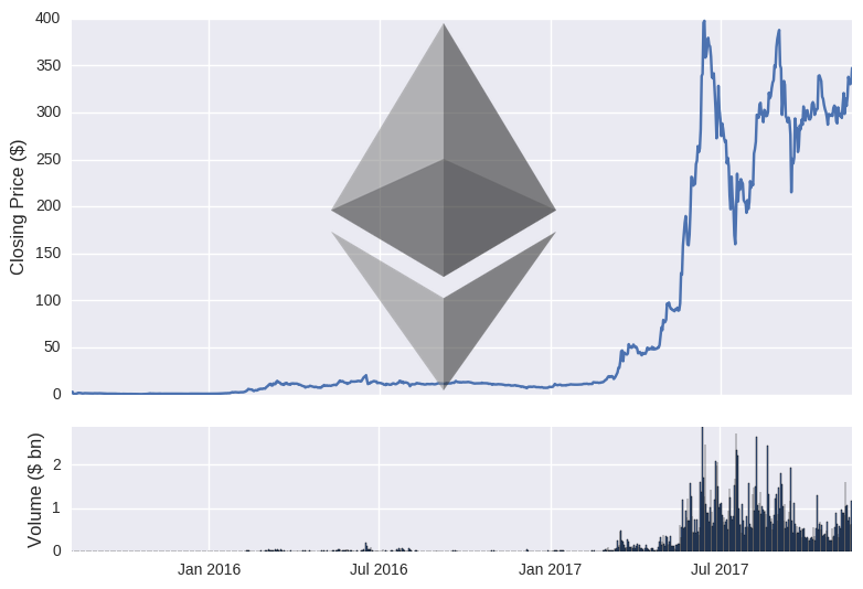
To prove that the data is accurate, we can plot the price and volume of both cryptos over time.
Training, Test & Random Walks
We have some data, so now we need to build a model. In deep learning, the data is typically split into training and test sets. The model is built on the training set and subsequently evaluated on the unseen test set. In time series models, we generally train on one period of time and then test on another separate period. Rather arbitrarily, I’ll set the cut-off date to June 1st 2017 (i.e. model will be trained on data before that date and assessed on data after it).
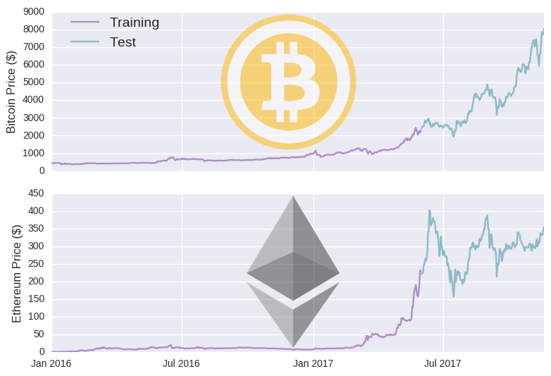
You can see that the training period mostly consists of periods when cryptos were relatively cheaper. As such, the training data may not be representative of the test data, undermining the model’s ability to generalise to unseen data (you could try to make your data stationary- discussed here). But why let negative realities get in the way of baseless optimism? Before we take our deep artificially intelligent machine learning model to the moon, it’s worth discussing a simpler model. The most basic model is to set tomorrow’s price equal to today’s price (which we’ll crudely call a lag model). This is how we’d define such a model in mathematical terms:
Extending this trivial lag model, stock prices are commonly treated as random walks, which can be defined in these mathematical terms:
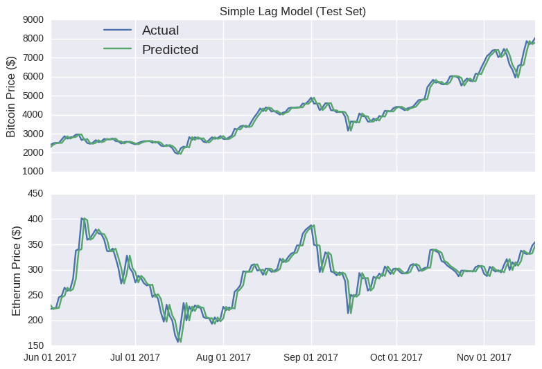
We’ll determine μ and σ from the training sets and apply the random walk model to the Bitcoin and Ethereum test sets.
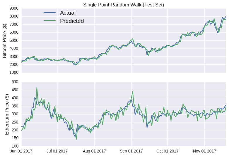
Wow! Look at those prediction lines. Apart from a few kinks, it broadly tracks the actual closing price for each coin. It even captures the eth rises (and subsequent falls) in mid-June and late August. At this stage, if I was to announce the launch of sheehanCoin, I’m sure that ICO would stupidly over-subscribed. As pointed out on that other blog, models that only make predictions one point into the future are often misleadingly accurate, as errors aren’t carried over to subsequent predictions. No matter how large the error, it’s essentially reset at each time point, as the model is fed the true price. The Bitcoin random walk is particularly deceptive, as the scale of the y-axis is quite wide, making the prediction line appear quite smooth.
Single point predictions are unfortunately quite common when evaluating time series models (e.g.here and here). A better idea could be to measure its accuracy on multi-point predictions. That way, errors from previous predictions aren’t reset but rather are compounded by subsequent predictions. Thus, poor models are penalised more heavily. In mathematical terms:
Let’s get our random walk model to predict the closing prices over the total test set.
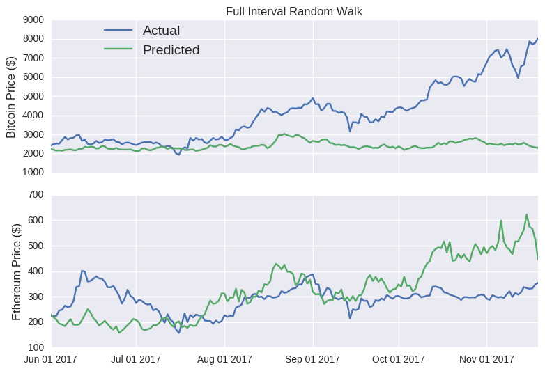
The model predictions are extremely sensitive to the random seed. I’ve selected one where the full interval random walk looks almost decent for Ethereum. In the accompanying Jupyter notebook, you can interactively play around with the seed value below to see how badly it can perform.
Notice how the single point random walk always looks quite accurate, even though there’s no real substance behind it. Hopefully, you’ll be more suspicious of any blog that claims to accurately predict prices. I probably shouldn’t worry; it’s not like crypto fans to be seduced by slick marketing claims.
Long Short Term Memory (LSTM)
Like I said, if you’re interested in the theory behind LSTMs, then I’ll refer you to this, this and this. Luckily, we don’t need to build the network from scratch (or even understand it), there exists packages that include standard implementations of various deep learning algorithms (e.g. TensorFlow, Keras, PyTorch, etc.). I’ll opt for Keras, as I find it the most intuitive for non-experts. If you’re not familiar with Keras, then check out my previous tutorial.
model_data.head()
| Date | bt_Close | bt_Volume | bt_close_off_high | bt_volatility | eth_Close | eth_Volume | eth_close_off_high | eth_volatility | |
|---|---|---|---|---|---|---|---|---|---|
| 688 | 2016-01-01 | 434.33 | 36278900 | -0.560641 | 0.020292 | 0.948024 | 206062 | -0.418477 | 0.025040 |
| 687 | 2016-01-02 | 433.44 | 30096600 | 0.250597 | 0.009641 | 0.937124 | 255504 | 0.965898 | 0.034913 |
| 686 | 2016-01-03 | 430.01 | 39633800 | -0.173865 | 0.020827 | 0.971905 | 407632 | -0.317885 | 0.060792 |
| 685 | 2016-01-04 | 433.09 | 38477500 | -0.474265 | 0.012649 | 0.954480 | 346245 | -0.057657 | 0.047943 |
| 684 | 2016-01-05 | 431.96 | 34522600 | -0.013333 | 0.010391 | 0.950176 | 219833 | 0.697930 | 0.025236 |
I’ve created a new data frame called model_data. I’ve removed some of the previous columns (open price, daily highs and lows) and reformulated some new ones. close_off_high represents the gap between the closing price and price high for that day, where values of -1 and 1 mean the closing price was equal to the daily low or daily high, respectively. The volatility columns are simply the difference between high and low price divided by the opening price. You may also notice that model_data is arranged in order of earliest to latest. We don’t actually need the date column anymore, as that information won’t be fed into the model.
Our LSTM model will use previous data (both bitcoin and eth) to predict the next day’s closing price of a specific coin. We must decide how many previous days it will have access to. Again, it’s rather arbitrary, but I’ll opt for 10 days, as it’s a nice round number. We build little data frames consisting of 10 consecutive days of data (called windows), so the first window will consist of the 0-9th rows of the training set (Python is zero-indexed), the second will be the rows 1-10, etc. Picking a small window size means we can feed more windows into our model; the downside is that the model may not have sufficient information to detect complex long term behaviours (if such things exist).
Deep learning models don’t like inputs that vary wildly. Looking at those columns, some values range between -1 and 1, while others are on the scale of millions. We need to normalise the data, so that our inputs are somewhat consistent. Typically, you want values between -1 and 1. The off_high and volatility columns are fine as they are. For the remaining columns, like that other blog post, we’ll normalise the inputs to the first value in the window.
| bt_Close | bt_Volume | bt_close_off_high | bt_volatility | eth_Close | eth_Volume | eth_close_off_high | eth_volatility | |
|---|---|---|---|---|---|---|---|---|
| 688 | 0.000000 | 0.000000 | -0.560641 | 0.020292 | 0.000000 | 0.000000 | -0.418477 | 0.025040 |
| 687 | -0.002049 | -0.170410 | 0.250597 | 0.009641 | -0.011498 | 0.239937 | 0.965898 | 0.034913 |
| 686 | -0.009946 | 0.092475 | -0.173865 | 0.020827 | 0.025190 | 0.978201 | -0.317885 | 0.060792 |
| 685 | -0.002855 | 0.060603 | -0.474265 | 0.012649 | 0.006810 | 0.680295 | -0.057657 | 0.047943 |
| 684 | -0.005457 | -0.048411 | -0.013333 | 0.010391 | 0.002270 | 0.066829 | 0.697930 | 0.025236 |
| 683 | -0.012019 | -0.061645 | -0.003623 | 0.012782 | 0.002991 | 0.498534 | -0.214540 | 0.026263 |
| 682 | 0.054613 | 1.413585 | -0.951499 | 0.069045 | -0.006349 | 2.142074 | 0.681644 | 0.040587 |
| 681 | 0.043515 | 0.570968 | 0.294196 | 0.032762 | 0.040890 | 1.647747 | -0.806717 | 0.055274 |
| 680 | 0.030576 | -0.110282 | 0.814194 | 0.017094 | 0.040937 | 0.098121 | -0.411897 | 0.019021 |
| 679 | 0.031451 | -0.007801 | -0.919598 | 0.017758 | 0.054014 | 0.896944 | -0.938235 | 0.025266 |
This table represents an example of our LSTM model input (we’ll actually have hundreds of similar tables). We’ve normalised some columns so that their values are equal to 0 in the first time point, so we’re aiming to predict changes in price relative to this timepoint. We’re now ready to build the LSTM model. This is actually quite straightforward with Keras, you simply stack componenets on top of each other (better explained here).
# import the relevant Keras modules
from keras.models import Sequential
from keras.layers import Activation, Dense
from keras.layers import LSTM
from keras.layers import Dropout

def build_model(inputs, output_size, neurons, activ_func = "linear",
                dropout =0.25, loss="mae", optimizer="adam"):
    model = Sequential()

    model.add(LSTM(neurons, input_shape=(inputs.shape[1], inputs.shape[2])))
    model.add(Dropout(dropout))

    model.add(Dense(units=output_size))
    model.add(Activation(activ_func))

    model.compile(loss=loss, optimizer=optimizer)
    return model
So, the build_model functions constructs an empty model unimaginatively called model (model = Sequential), to which an LSTM layer is added. That layer has been shaped to fit our inputs (n x m tables, where n and m represent the number of timepoints/rows and columns, respectively). The function also includes more generic neural network features, like dropout and activation functions. Now, we just need to specify the number of neurons to place in the LSTM layer (I’ve opted for 20 to keep runtime reasonable), as well as the data on which the model will be trained.
# random seed for reproducibility
np.random.seed(202)
# initialise model architecture
eth_model = build_model(LSTM_training_inputs, output_size=1, neurons = 20)
# model output is next price normalised to 10th previous closing price
LSTM_training_outputs = (training_set['eth_Close'][window_len:].values/training_set['eth_Close'][:-window_len].values)-1
# train model on data
# note: eth_history contains information on the training error per epoch
eth_history = eth_model.fit(LSTM_training_inputs, LSTM_training_outputs,
                            epochs=50, batch_size=1, verbose=2, shuffle=True)
#eth_preds = np.loadtxt('eth_preds.txt')
Epoch 50/50
6s - loss: 0.0625
We’ve just built an LSTM model to predict tomorrow’s Ethereum closing price. Let’s see how well it performs. We start by examining its performance on the training set (data before June 2017). That number below the code represents the model’s mean absolute error (mae) on the training set after the 50th training iteration (or epoch). Instead of relative changes, we can view the model output as daily closing prices.
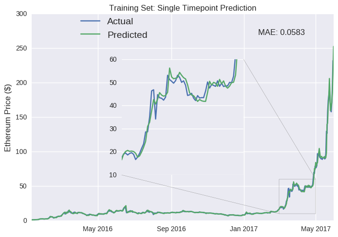
We shouldn’t be too surprised by its apparent accuracy here. The model could access the source of its error and adjust itself accordingly. In fact, it’s not hard to attain almost zero training errors. We could just cram in hundreds of neurons and train for thousands of epochs (a process known as overfitting, where you’re essentially predicting noise- I included the Dropout() call in the build_model function to mitigate this risk for our relatively small model). We should be more interested in its performance on the test dataset, as this represents completely new data for the model.
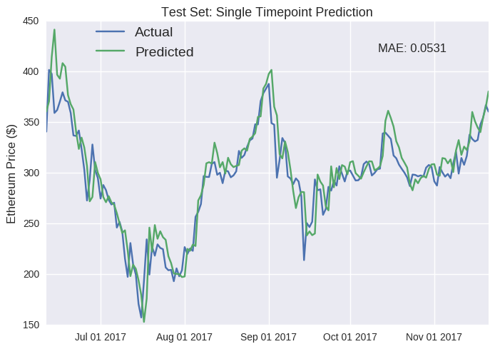
Caveats aside about the misleading nature of single point predictions, our LSTM model seems to have performed well on the unseen test set. The most obvious flaw is that it fails to detect the inevitable downturn when the eth price suddenly shoots up (e.g mid-June and October). In fact, this is a persistent failure; it’s just more apparent at these spikes. The predicted price regularly seems equivalent to the actual price just shifted one day later (e.g. the drop in mid-July). Furthermore, the model seems to be systemically overestimating the future value of Ether (join the club, right?), as the predicted line near always runs higher than the actual line. I suspect this is because the training data represents a period during which the price of Ether rose astronomically, so it expects that trend to continue (don’t we all). We can also build a similar LSTM model for Bitcoin- test set predictions are plotted below (see Jupyter notebook for full code).
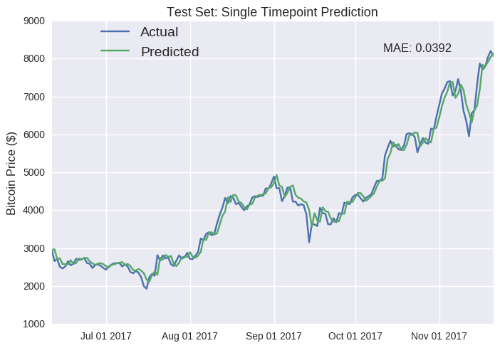
As I’ve stated earlier, single point predictions can be deceptive. Looking more closely, you’ll notice that, again, the predicted values regularly mirror the previous values (e.g. October). Our fancy deep learning LSTM model has partially reproducted a autregressive (AR) model of some order p, where future values are simply the weighted sum of the previous p values. We can define an AR model in these mathematical terms:
The good news is that AR models are commonly employed in time series tasks (e.g. stock market prices), so the LSTM model appears to have landed on a sensible solution. The bad news is that it’s a waste of the LSTM capabilities, we could have a built a much simpler AR model in much less time and probably achieved similar results (though the title of this post would have been much less clickbaity). More complex does not automatically equal more accurate.
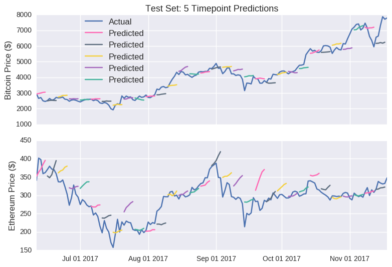
The predictions are visibly less impressive than their single point counterparts. Nevertheless, I’m pleased that the model returned somewhat nuanced behaviours (e.g. the second line on the eth graph); it didn’t simply forecast prices to move uniformly in one direction. So there are some grounds for optimism.
Moving back to the single point predictions, our deep machine artificial neural model looks okay, but so did that boring random walk model. Like the random walk model, LSTM models can be sensitive to the choice of random seed (the model weights are initially randomly assigned). So, if we want to compare the two models, we’ll run each one multiple (say, 25) times to get an estimate for the model error. The error will be calculated as the absolute difference between the actual and predicted closing prices changes in the test set.
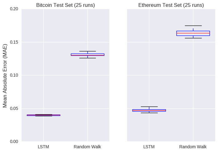
Maybe AI is worth the hype after all! Those graphs show the error on the test set after 25 different initialisations of each model. The LSTM model returns an average error of about 0.04 and 0.05 on the bitcoin and eth prices, respectively, crushing the corresponding random walk models.
Aiming to beat random walks is a pretty low bar. It would be more interesting to compare the LSTM model against more appropriate time series models (weighted average, autoregression, ARIMA or Facebook’s Prophet algorithm). On the other hand, I’m sure it wouldn’t be hard to improve our LSTM model (gratuitously adding more layers and/or neurons, changing the batch size, learning rate, etc.). That said, hopefully you’ve detected my scepticism when it comes to applying deep learning to predict changes in crypto prices. That’s because we’re overlooking the best framework of all: human intelligence. Clearly, the perfect model* for predicting cryptos is:
* This blog does not constitute financial advice and should not be taken as such. While cryptocurrency investments will definitely go up in value forever, they may also go down.
Summary
We’ve collected some crypto data and fed it into a supercool deeply intelligent machine learning LSTM model. Unfortunately, its predictions were not that different from just spitting out the previous value. How can we make the model learn more sophisticated behaviours?
-
Change Loss Function: MAE doesn’t really encourage risk taking. For example, under mean squared error (MSE), the LSTM model would be forced to place more importance on detecting spikes/troughs. More bespoke trading focused loss functions could also move the model towards less conservative behaviours.
-
Penalise conservative AR-type models: This would incentivise the deep learning algorithm to explore more risky/interesting models. Easier said than done!
-
Get more and/or better data: If past prices alone are sufficient to decently forecast future prices, we need to include other features that provide comparable predictive power. That way, the LSTM model wouldn’t be so reliant on past prices, potentially unlocking more complex behaviours. This is probably the best and hardest solution.
If that’s the positive spin, then the negative reality is that it’s entirely possible that there is no detectable pattern to changes in crypto prices; that no model (however deep) can separate the signal from the noise (similar to the merits of using deep learning to predict earthquakes). And any pattern that does appear can disappear as quickly (see efficient market hypothesis). Just think how different Bitcoin in 2016 is to craze-riding Bitcoin of late 2017. Any model built on 2016 data would surely struggle to replicate these unprecedented movements. All of this suggests you might as well save yourself some time and stick to autoregression (unless you’re writing a blog, of course).
But I’m sure they’ll eventually find some use cases for deep learning. In the meantime, you can build your own LSTM model by downloading the Python code here. Thanks for reading!
Leave a Comment